Stochastic matrix

From Wikipedia, the free encyclopedia

Jump to: navigation, search

For a matrix whose elements are stochastic, see Random matrix

In mathematics, a stochastic matrix (also termed probability matrix, transition matrix, substitution matrix, or Markov matrix) is a matrix used to describe the transitions of a Markov chain. It has found use in probability theory, statistics and linear algebra, as well as computer science. There are several different definitions and types of stochastic matrices;

A right stochastic matrix is a square matrix each of whose rows consists of nonnegative real numbers, with each row summing to 1.

A left stochastic matrix is a square matrix each of whose columns consist of nonnegative real numbers, with each column summing to 1.

A doubly stochastic matrix is a square matrix where all entries are nonnegative and all rows and all columns sum to 1.

In the same vein, one may define a stochastic vector as a vector whose elements consist of nonnegative real numbers which sum to 1. Thus, each row (or column) of a stochastic matrix is a probability vector, which are sometimes called stochastic vectors.
A common convention in English language mathematics literature is to use row vectors of probabilities and right stochastic matrices rather than column vectors of probabilities and left stochastic matrices; this article follows that convention.

Definition and properties

A stochastic matrix describes a Markov chain $\boldsymbol{X}_{t}$ over a finite state space S.
If the probability of moving from $i$ to $j$ in one time step is $Pr(j|i)=P_{i,j}$ , the stochastic matrix P is given by using $P_{i,j}$ as the $i^{th}$ row and $j^{th}$ column element, e.g.,

$P=\left(\begin{matrix}p_{1,1}&p_{1,2}&\dots&p_{1,j}&\dots\\ p_{2,1}&p_{2,2}&\dots&p_{2,j}&\dots\\ \vdots&\vdots&\ddots&\vdots&\ddots\\ p_{i,1}&p_{i,2}&\dots&p_{i,j}&\dots\\ \vdots&\vdots&\ddots&\vdots&\ddots \end{matrix}\right).$

Since the probability of transitioning from state $i$ to some state must be 1, this matrix is a right stochastic matrix, so that

$\sum_j P_{i,j}=1.\,$

The probability of transitioning from $i$ to $j$ in two steps is then given by the $(i,j)^{th}$ element of the square of $P$ :

$\left(P ^{2}\right)_{i,j}.$

In general the probability transition of going from any state to another state in a finite Markov chain given by the matrix $P$ in k steps is given by $P^k$ .
An initial distribution is given as a row vector.
A stationary probability vector $\boldsymbol{\pi}$ is defined as a vector that does not change under application of the transition matrix; that is, it is defined as a left eigenvector of the probability matrix, associated with eigenvalue 1:

$\boldsymbol{\pi}P=\boldsymbol{\pi}.$

The Perron–Frobenius theorem ensures that every stochastic matrix has such a vector, and that the largest absolute value of an eigenvalue is always 1. In general, there may be several such vectors. However, for a matrix with strictly positive entries, this vector is unique and can be computed by observing that for any $i$ we have the following limit,

$\lim_{k\rightarrow\infty}\left(P^k \right)_{i,j}=\boldsymbol{\pi}_j,$

where $\boldsymbol{\pi}_{j}$ is the $j^{th}$ element of the row vector $\boldsymbol{\pi}$ . This implies that the long-term probability of being in a state $j$ is independent of the initial state $i$ . That either of these two computations give one and the same stationary vector is a form of an ergodic theorem, which is generally true in a wide variety of dissipative dynamical systems: the system evolves, over time, to a stationary state. Intuitively, a stochastic matrix represents a Markov chain with no sink states, this implies that the application of the stochastic matrix to a probability distribution would redistribute the probability mass of the original distribution while preserving its total mass. If this process is applied repeatedly the distribution converges to a stationary distribution for the Markov chain.

Example: the cat and mouse

Suppose you have a timer and a row of five adjacent boxes, with a cat in the first box and a mouse in the fifth box at time zero. The cat and the mouse both jump to a random adjacent box when the timer advances. E.g. if the cat is in the second box and the mouse in the fourth one, the probability is one fourth that the cat will be in the first box and the mouse in the fifth after the timer advances. If the cat is in the first box and the mouse in the fifth one, the probability is one that the cat will be in box two and the mouse will be in box four after the timer advances. The cat eats the mouse if both end up in the same box, at which time the game ends. The random variable K gives the number of time steps the mouse stays in the game.
The Markov chain that represents this game contains the following five states:

State 1: cat in the first box, mouse in the third box: (1, 3)
State 2: cat in the first box, mouse in the fifth box: (1, 5)
State 3: cat in the second box, mouse in the fourth box: (2, 4)
State 4: cat in the third box, mouse in the fifth box: (3, 5)
State 5: the cat ate the mouse and the game ended: F.

We use a stochastic matrix to represent the transition probabilities of this system,

$P = \begin{bmatrix} 0 & 0 & 1/2 & 0 & 1/2 \\ 0 & 0 & 1 & 0 & 0 \\ 1/4 & 1/4 & 0 & 1/4 & 1/4 \\ 0 & 0 & 1/2 & 0 & 1/2 \\ 0 & 0 & 0 & 0 & 1 \end{bmatrix}.$

Long-term averages

As state 5 is an absorbing state the long-term average vector $\boldsymbol{\pi}=(0,0,0,0,1)$ . Regardless of the initial conditions the cat will eventually catch the mouse.

Phase-type representation

The survival function of the mouse. Note the mouse will survive at least the first time step.

As the game has an absorbing state 5 the distribution of time to absorption is discrete phase-type distributed. Suppose the system starts in state 2, represented by the vector $[0,1,0,0,0]$ . To simplify the calculations, state five can be ignored. Let

$\boldsymbol{\tau}=[0,1,0,0]$

and remove state five to make a sub-stochastic matrix,

$T=\begin{bmatrix} 0 & 0 & 1/2 & 0\\ 0 & 0 & 1 & 0\\ 1/4 & 1/4 & 0 & 1/4\\ 0 & 0 & 1/2 & 0\\ \end{bmatrix}\,,$ with $(I-T)^{-1}\boldsymbol{1} =\begin{bmatrix}2.75 \\ 4.5 \\ 3.5 \\ 2.75\end{bmatrix}\,,$

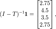
where $I$ is the identity matrix, and $\mathbf{1}$ represents a column matrix of all ones. The expected time of the mouse's survival is given by

$E[K]=\boldsymbol{\tau}(I-T)^{-1}\boldsymbol{1}=4.5.$

Higher order moments are given by

$E[K(K-1)\dots(K-n+1)]=n!\boldsymbol{\tau}(I-{T})^{-n}{T}^{n-1}\mathbf{1}\,.$

References

G. Latouche, V. Ramaswami. Introduction to Matrix Analytic Methods in Stochastic Modeling, 1st edition. Chapter 2: PH Distributions; ASA SIAM, 1999.

A Data Scientist's blog

Search This Blog

Wednesday, June 06, 2012