Search This Blog

Sunday, February 12, 2012

EM algorithm starting with E-step for parameterized Gaussian mixture models


em {mclust}R Documentation

EM algorithm starting with E-step for parameterized Gaussian mixture models.

Description

Implements the EM algorithm for parameterized Gaussian mixture models, starting with the expectation step.

Usage

em(modelName, data, parameters, prior = NULL, control = emControl(),
   warn = NULL, ...)

Arguments

modelName A character string indicating the model. The help file for mclustModelNames describes the available models.
data A numeric vector, matrix, or data frame of observations. Categorical variables are not allowed. If a matrix or data frame, rows correspond to observations and columns correspond to variables.
parameters A names list giving the parameters of the model. The components are as follows:
pro
Mixing proportions for the components of the mixture. If the model includes a Poisson term for noise, there should be one more mixing proportion than the number of Gaussian components.
mean
The mean for each component. If there is more than one component, this is a matrix whose kth column is the mean of the kth component of the mixture model.
variance
A list of variance parameters for the model. The components of this list depend on the model specification. See the help file for mclustVariance for details.
Vinv
An estimate of the reciprocal hypervolume of the data region. If set to NULL or a negative value, the default is determined by applying function hypvol to the data. Used only when pro includes an additional mixing proportion for a noise component.
prior Specification of a conjugate prior on the means and variances. The default assumes no prior.
control A list of control parameters for EM. The defaults are set by the call emControl().
warn A logical value indicating whether or not a warning should be issued when computations fail. The default is warn=FALSE.
... Catches unused arguments in indirect or list calls via do.call.

Value

A list including the following components:
modelName A character string identifying the model (same as the input argument).
z A matrix whose [i,k]th entry is the conditional probability of the ith observation belonging to the kth component of the mixture.
parameters
pro
A vector whose kth component is the mixing proportion for the kth component of the mixture model. If the model includes a Poisson term for noise, there should be one more mixing proportion than the number of Gaussian components.
mean
The mean for each component. If there is more than one component, this is a matrix whose kth column is the mean of the kth component of the mixture model.
variance
A list of variance parameters for the model. The components of this list depend on the model specification. See the help file for mclustVariance for details.
Vinv
The estimate of the reciprocal hypervolume of the data region used in the computation when the input indicates the addition of a noise component to the model.
loglik The log likelihood for the data in the mixture model.
Attributes:
    "info"
    Information on the iteration.
    "WARNING"
    An appropriate warning if problems are encountered in the computations.

References

C. Fraley and A. E. Raftery (2002). Model-based clustering, discriminant analysis, and density estimation. Journal of the American Statistical Association 97:611-631.
C. Fraley and A. E. Raftery (2005). Bayesian regularization for normal mixture estimation and model-based clustering. Technical Report, Department of Statistics, University of Washington.
C. Fraley and A. E. Raftery (2006). MCLUST Version 3 for R: Normal Mixture Modeling and Model-Based Clustering, Technical Report no. 504, Department of Statistics, University of Washington.

See Also

emE, ..., emVVV, estep, me, mstep, mclustOptions, do.call

Examples

msEst <- mstep(modelName = "EEE", data = iris[,-5], 
               z = unmap(iris[,5]))
names(msEst)

em(modelName = msEst$modelName, data = iris[,-5],
   parameters = msEst$parameters)
## Not run: 
do.call("em", c(list(data = iris[,-5]), msEst))   ## alternative call
## End(Not run)

[Package mclust version 3.1-1 Index]

EM algorithm for incomplete categorical data


em.cat {cat}R Documentation

EM algorithm for incomplete categorical data

Description

Finds ML estimate or posterior mode of cell probabilities under the saturated multinomial model.

Usage

em.cat(s, start, prior=1, showits=T, maxits=1000,
eps=0.0001)

Arguments

s summary list of an incomplete categorical dataset produced by the function prelim.cat.
start optional starting value of the parameter. This is an array with dimensions s$d whose elements sum to one. The default starting value is a uniform array (equal probabilities in all cells). If structural zeros appear in the table, start should contain zeros in those positions and nonzero (e.g. uniform) values elsewhere.
prior optional vector of hyperparameters for a Dirichlet prior distribution. The default is a uniform prior distribution (all hyperparameters = 1) on the cell probabilities, which will result in maximum likelihood estimation. If structural zeros appear in the table, a prior should be supplied with NAs in those cells.
showits if TRUE, reports the iterations of EM so the user can monitor the progress of the algorithm.
maxits maximum number of iterations performed. The algorithm will stop if the parameter still has not converged after this many iterations.
eps convergence criterion. This is the largest proportional change in an expected cell count from one iteration to the next. Any expected cell count that drops below 1E-07 times the average cell probability (1/number of non-structural zero cells) is set to zero during the iterations.

Value

array of dimension s$d containing the ML estimate or posterior mode, assuming that EM has converged by maxits iterations.

Note

If zero cell counts occur in the observed-data table, the maximum likelihood estimate may not be unique, and the algorithm may converge to different stationary values depending on the starting value. Also, if zero cell counts occur in the observed-data table, the ML estimate may lie on the boundary of the parameter space. Supplying a prior with hyperparameters greater than one will give a unique posterior mode in the interior of the parameter space. Estimated probabilities for structural zero cells will always be zero.

References

Schafer (1996) Analysis of Incomplete Multivariate Data. Chapman & Hall, Section 7.3.

See Also

prelim.cat, ecm.cat, logpost.cat

Examples

data(crimes)
crimes
s <- prelim.cat(crimes[,1:2],crimes[,3])     # preliminary manipulations
thetahat <- em.cat(s)                        # mle under saturated model
logpost.cat(s,thetahat)                      # loglikelihood at thetahat

Data Mining Algorithms In R/Clustering/Expectation Maximization (EM)

Data Mining Algorithms In R/Clustering/Expectation Maximization (EM)

< Data Mining Algorithms In R | Clustering
This chapter intends to give an overview of the technique Expectation Maximization (EM), proposed by [1] (although the technique was informally proposed in literature, as suggested by the author) in the context of R-Project environment. The first section gives an introduction of representative clustering and mixture models. The algorithm details and a case study will be presented on the second section.
The R package that will be used is the MCLUST-v3.3.2 developed by Chris Fraley and Adrian Raftery, available in CRAN repository. The MCLUST tool is a software that includes the following features: normal mixture modeling (EM); EM initialization through an hierarquical clustering approach; estimate the number of clusters based on the Bayesian Information Criteria (BIC); and displays, including uncertainty plots and dimension projections.
The information sources of this document were divided in two groups: (i) manual and guides of R and MCLUST, which includes the technical report [2] that is the base reference of this project and gives an overview of MCLUST with several examples and (ii) theoretical papers, surveys and books found in literature.

Contents

 [hide

[edit] Introduction

Clustering consists in identifying groups of entities that have characteristics in common and are cohesive and separated from each other. Interest in clustering has increased due to several applications in distinct knowledge areas. Highlighting the search for grouping of customers and products in massive datasets, document analysis in Web usage data, gene expression from microarrays and image analysis where clustering is used for segmentation.
The clustering methods can be grouped in classes. One widely used involves hierarchical clustering, which consider, initially, that each points represent one group and at each iteration it merged two groups chosen to optimize some criterion. A popular criteria, proposed by [3], include the sum of within group sum of squares and is given by the shortest distance between the groups (single-link method).
Another typical class is based on iterative relocation, which data are moved from one group to another at each iteration. Also called as representative clustering due the use of a model, created to each cluster, that summarize the characteristics of the group elements. The most popular method in this class is the K-Means, proposed by [4], which is based on iterative relocation with the sum of squares criterion.
In statistic and optimization problems is usual maximize or minimize a function, and its variables in a specific space. As these optimization problems may assume several different types, each one with its own characteristics, many techniques have been developed to solve them. This techniques are very important in data mining and knowledge discovery area as it can be used as basis for most complex and powerful methods.
One of these techniques is the Maximum Likelihood and its main goal is to adjust a statistic model with a specific data set, estimating its unknown parameters so the function that can describe all the parameters in the dataset. In other words, the method will adjust some variables of a statistical model from a dataset or a known distribution, so the model can “describe” each data sample and estimate others.
It was realized that clustering can be based on probability models to cover the missing values. This provides insights into when the data should conform to the model and has led to the development of new clustering methods such as Expectation Maximization (EM) that is based on the principle of Maximum Likelihood of unobserved variables in finite mixture models.

[edit] Technique to be discussed

The EM algorithm is an unsupervised clustering method, that is, don't require a training phase, based on mixture models. It follows an iterative approach, sub-optimal, which tries to find the parameters of the probability distribution that has the maximum likelihood of its attributes.
In general lines, the algorithm's input are the data set (x), the total number of clusters (M), the accepted error to converge (e) and the maximum number of iterations. For each iteration, first is executed the E-Step (E-xpectation), that estimates the probability of each point belongs to each cluster, followed by the M-step (M-aximization), that re-estimate the parameter vector of the probability distribution of each class. The algorithm finishes when the distribution parameters converges or reach the maximum number of iterations.

[edit] Algorithm

Initialization
Each classe j, of M classes (or clusters), is constituted by a parameter vector (θ), composed by the mean (μj) and by the covariance matrix (Pj), which represents the features of the Gaussian probability distribution (Normal) used to characterize the observed and unobserved entities of the data set x.

\theta(t) = { \mu_j(t),\ P_j(t) },\ j\ =\ 1..M
On the initial instant (t = 0) the implementation can generate randomly the initial values of mean (μj) and of covariance matrix (Pj). The EM algorithm aims to approximate the parameter vector (θ) of the real distribution. Another alternative offered by MCLUST is to initialize EM with the clusters obtained by a hierarquical clustering technique.
E-Step
This step is responsible to estimate the probability of each element belong to each cluster (P(Cj | xk) ). Each element is composed by an attribute vector (xk). The relevance degree of the points of each cluster is given by the likelihood of each element attribute in comparison with the attributes of the other elements of cluster Cj.

P(C_j|x) = \frac{|\sum_j(t)|^{-\frac{1}{2}}\ exp^{n_j}\ P_j(t)}{\sum_{k=1}^M\ |\sum_j(t)|^{-\frac{1}{2}}\ exp^{n_j}\ P_k(t)}
M-Step
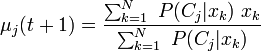
This step is responsible to estimate the parametrs of the probability distribution of each class for the next step. First is computed the mean (μj) of classe j obtained through the mean of all points in function of the relevance degree of each point.

\mu_j(t+1) = \frac{\sum_{k=1}^N\ P(C_j|x_k)\ x_k}{\sum_{k=1}^N\ P(C_j|x_k)}
To compute the covariance matrix for the next iteration is applied the Bayes Theorem, which implies that P(A | B) = P(B | A) * P(A)P(B), based on the conditional probabilities of the class occurrence.
 
\sum_j(t+1) = \frac{\sum_{k=1}^N\ P(C_j|x_k)\ (x_k - \mu_j(t) )\ (x_k - \mu_j(t) )}{\sum_{k=1}^N\ P(C_j|x_k)}
The probability of occurrence of each class is computed through the mean of probabilities (Cj) in function of the relevance degree of each point from the class.
 
P_j(t+1) = \frac{1}{N} \sum_{k=1}^N P(C_j|x_k)
The attributes represents the parameter vector θ that characterize the probability distribution of each class that will be used in the next algorithm iteration.
Convergence Test
After each iteration is performed a convergence test which verifies if the difference of the attributes vector of an iteration to the previous iteration is smaller than an acceptable erro tolerance, given by parameter. Some implementations uses the difference between the averages of class distribution as the convergence criterion.
if(||θ(t + 1) − θ(t)|| < ǫ)
   stop
else
   call E-Step
end

The algorithm has the property of, at each step, estimate a new attribute vector that has the maximum local likelihood, not necessarily the global, what reduces the its complexity. However, depending on the dispersion of the data and on its volume, the algorithm can stop due the maximum number of iterations defined.

[edit] Implementation

[edit] Packages

The expectation-maximization in algorithm in R [5], proposed in [6], will use the package mclust. This package contains crucial methods for the execution of the clustering algorithm, including functions for the E-step and M-step calculation. The package manual explains all of its functions, including simple examples. This manual can be found in [2][6].
The mclust package also provides various models for EM and also hierarchical clustering(HC), which is defined by the covariance structures. These models are presented in Table 1 and are explained in detail in [7].
Table 1: Covariance matrix structures.
identifier Model HC EM Distribution Volume Shape Orientation
E
* * (univariate) equal

V
* * (univariate) variable

EII λI * * Spherical equal equal NA
VII λkI * * Spherical variable equal NA
EEI λA
* Diagonal equal equal coordinate axes
VEI λkA
* Diagonal variable equal coordinate axes
EVI λAk
* Diagonal equal variable coordinate axes
VVI λkAk
* Diagonal variable variable coordinate axes
EEE λDADT * * Ellipsoidal equal equal equal
EEV \lambda D_k A D_k^T
* Ellipsoidal equal equal variable
VEV \lambda_k D_k A D_k^T
* Ellipsoidal variable equal variable
VVV \lambda_k D_k A_k D_k^T * * Ellipsoidal variable variable variable

[edit] Executing the Algorithm

The function “em” can be used for the expectation-maximization method, as it implements the method for parameterized Gaussian Mixture Models (GMM), starting in the E-step. This function uses the following parameters:
  • model-name: the name of the model used;
  • data: all the collected data, which must be all numerical. If the data format is represent by a matrix, the rows will represent the samples (observations) and the columns the variables;
  • parameters: model parameters, which can assume the following values: pro, mean, variance and Vinv, corresponding to the mixture proportion for the components of mixture, mean of each component, parameters variance and the estimate hypervolume of the data region, respectively.
  • other: less relevant parameters which wont be described here. More details can be found in the package manual.
After the execution, the function will return:
  • model-name: the name of the model;
  • z: a matrix whose the element in position [I,k] presents the conditional probability of the ith sample belongs to the kth mixture component;
  • parameters: same as the input;
  • others: other metrics which wont be discussed here. More details can be found in the package manual.

[edit] A simple example

In order to demonstrate how to use the R to execute the expectation-Maximization method, the following algorithm presents a simple example for a test dataset. This example can also be found in the package manual.
> modelName = ``EEE''
> data = iris[,-5]
> z = unmap(iris[,5])
> msEst <- mstep(modelName, data, z)
> names(msEst)
> modelName = msEst$modelName
> parameters = msEst$parameters
> em(modelName, data, parameters)
The first line executes the M-step so the parameters used in the em function can be generated. This function is called mstep and its inputs are model name, as “EEE”, the dataseta the iris dataset and finally, the z matrix, which contains the conditional probability of each class contains each data sample. This z matrix is generated by the unmap function.
After the M-step, the algorithm will show (line 2) the attributes of the object returned by this function. The third line will start the clustering process using some of the result of the M-step method as input.
The clustering method will return the parameters estimated in the process and the conditional probability of each sample falls in each class. These parameters include mean and variance, and this last one corresponds to the use of the mclustVariance method.

[edit] View

This section will present some examples of visualization available in MCLUST package. First will be showed a simple example of the overall process of clustering from the choice of the number of clusters, the initialization and the partitioning. Then it will be explained a didactical example using two random mixtures in comparison with two gaussian mixtures.
Basic Example
This is a simple example to show the features offered by MCLUST package. It is applied to the faithful dataset (included in R project). First the cluster analysis estimates the number of clusters that best represents this data set and also the covariance structure of the spread points. This is performed through the technique called Bayesian Information Criterion (BIC) that varies the number of cluster from 1 to 9. The BIC is the value of the maximized loglikelihood measured with a penalty for the number of parameters in the model. Then it's executed the hierarchical clustering technique (HC), which doesn't require a initialization phase. The output of the HC, that is, the cluster that each element belongs, is used to initialize the Expectation-Maximization technique (EM). After the execution of EM clustering the charts are showed below:
### basic_example.R ###
# usage: R --no-save < basic_example.R

library(mclust)           # load mclust library
x = faithful[,1]          # get the first column of the faithful data set
y = faithful[,2]          # get the first column of the faithful data set
plot(x,y)                 # plot the spread points before the clustering
model <- Mclust(faithful) # estimate the number of cluster (BIC), initialize (HC) and clusterize (EM)
data = faithful           # get the data set 
plot(model, faithful)     # plot the clustering results

File:Basic points.pdf Basic bic.pdf Basic cluster.pdf Basic uncertainty.pdf Basic density.pdf
Didactical Example
A didactical example is developed to show two distinct scenarios: (a) one that the model doesn't represents the data and (b) another that the data is conformed to the model. This example intends to show how EM behaves with noised and clean data sets.
a) Uniform random mixtures
A noised data set is generated through a uniform random function. The points spread are showed in a chart. Then the clustering analysis is executed with default parameters (i.e. varies cluster from 1 to 9). The clustering tool shows a warning with a message that the best model occurs at the min or max, in this case is the min that all points are grouped in a single cluster.
### random_example.R ###
# usage: R --no-save < random_example.R

library(mclust)                  # load mclust library
x1 = runif(20)                   # generate 20 random random numbers for x axis (1st class)
y1 = runif(20)                   # generate 20 random random numbers for y axis (1st class)
x2 = runif(20)                   # generate 20 random random numbers for x axis (2nd class)
y2 = runif(20)                   # generate 20 random random numbers for y axis (2nd class)
rx = range(x1,x2)                # get the axis x range
ry = range(y1,y2)                # get the axis y range
plot(x1, y1, xlim=rx, ylim=ry)   # plot the first class points
points(x2, y2 )                  # plot the second class points
mix = matrix(nrow=40, ncol=2)    # create a dataframe matrix 
mix[,1] = c(x1, x2)              # insert first class points into the matrix
mix[,2] = c(y1, y2)              # insert second class points into the matrix
mixclust = Mclust(mix)           # initialize EM with hierarchical clustering, execute BIC and EM

# Warning messages:
# 1: In summary.mclustBIC(Bic, data, G = G, modelNames = modelNames) :
#    best model occurs at the min or max # of components considered
# 2: In Mclust(mix) : optimal number of clusters occurs at min choice


Points random.pdf
b) Two gaussian mixtures
This scenario is composed by two well separated data sets generated through a gaussian distribution function (Normal). The points are showed in the first chart. The EM clustering is applied and the results are also showed in the graphs below. As we can see, the EM clustering obtain two gaussian models that is in conformed to the data.
### gaussian_example.R ###
# usage: R --no-save < gaussian_example.R

library(mclust)                  # load mclust library
x1 = rnorm(n=20, mean=1, sd=1)   # get 20 normal distributed points for x axis with mean=1 and std=1 (1st class)
y1 = rnorm(n=20, mean=1, sd=1)   # get 20 normal distributed points for x axis with mean=1 and std=1 (2nd class)
x2 = rnorm(n=20, mean=5, sd=1)   # get 20 normal distributed points for x axis with mean=5 and std=1 (1st class)
y2 = rnorm(n=20, mean=5, sd=1)   # get 20 normal distributed points for x axis with mean=5 and std=1 (2nd class)
rx = range(x1,x2)                # get the axis x range
ry = range(y1,y2)                # get the axis y range
plot(x1, y1, xlim=rx, ylim=ry)   # plot the first class points
points(x2, y2)                   # plot the second class points
mix = matrix(nrow=40, ncol=2)    # create a dataframe matrix 
mix[,1] = c(x1, x2)              # insert first class points into the matrix
mix[,2] = c(y1, y2)              # insert second class points into the matrix
mixclust = Mclust(mix)           # initialize EM with hierarchical clustering, execute BIC and EM
plot(mixclust, data = mix)       # plot the two distinct clusters found 

Gaussian points.pdf Gaussian bic.pdf Gaussian cluster.pdf File:Gaussian density.pdf File:Gaussian uncertainty.pdf

[edit] Case Study

[edit] Scenario

The scenario to be analized is composed by a sample data set available in the MCLUST package named "wreath". A clustering analysis is performed with more details, applied to a scenario composed by 14 point groups, that exceeds the maximum number of clusters allowed by the default MCLUST parameters. The clustering technique is executed two times: (i) the first based on the default MCLUST, (ii) with customized parameters.

[edit] Input data

The input of the case study is the data set wreath provided by the MCLUST package. This data set consists in a 14 point group showed on the next figure, which can be modeled with Spherical or Ellipsoide that take into account the orientation of the data due its rotation.
### case_input.R ###
# usage: R --no-save < case_default.R

plot(wreath[,1],wreath[,2])


[edit] Execution

The clustering is executed two times. The first one is based on the default parameters given by the MCLUST tool, that varies the number of cluster from 1 to 9, which is smaller than the necessary to fit the case study data set. The estimation of the number of clusters is showed in a graphic that varies the number of clusters and compute the Bayesian Informatin Criterion (BIC) for each value. We can see that the BIC, using the default parameters, is divergent while is expected find a peak followed by a decrease that indicates the best number of clusters.
### case_default.R ###
# usage: R --no-save < case_default.R

library(mclust)

wreathBIC <- mclustBIC(wreath)
plot(wreathBIC, legendArgs = list(x = "topleft"))

Default bic.pdf
Then the number of cluster is customized, modified to varies from 1 to 20 as showed below. The BIC technique will give the best number of clusters, in this case 14 clusters and the coefficient structure that have the properties of this data set, that is the EEV, which means that the clusters has similar shape, similar volumes but variable orientation. After executes the BIC method again we can see that 14 clusters, indicated by the peak on the graphic, is the number of cluster that present the maximum likelihood for this data.
### case_customized.R ###
# usage: R --no-save < case_customized.R

library(mclust)
wreathDefault <- mclustBIC(wreath)
wreathCustomize <- mclustBIC(wreath, G = 1:20, x = wreathDefault)
plot(wreathBIC, G = 10:20, legendArgs = list(x = "bottomleft"))
summary(wreathBIC, wreath)

Customize bic.pdf

[edit] Output

The output of this clustering is analysed is obtained using the method mclust2Dplot depicted in the next figure. It was used the density visualization. The clusters found are characterized by 14 models wich have the distribution of an ellipsoides, with different orientation, beein in conformed with the data. The method summary can be executed later analyse other aspects of the clustering result.
### case_output.R ###
# usage: R --no-save < case_customized.R

library(mclust)
data(wreath)
wreathBIC <- mclustBIC(wreath)
wreathBIC <- mclustBIC(wreath, G = 1:20, x = wreathBIC)
wreathModel <- summary(wreathBIC, data = wreath)
mclust2Dplot(data = wreath, what = "density", identify = TRUE, parameters = wreathModel$parameters, z = wreathModel$z)

Cluster customize.pdf

[edit] Analysis

We can see that the mixture models created to represent the point are in conformation to the data set. On this case, the groups doesn't have an intersection between them, so all points were classified to the right group. The cluster orientation allows the method to find a better Ellipsoide to represent those points.
We conclude that the EM clustering technique, despite the dependence of the number of clusters and the initialization phase, is an efficient method that produces good results for several scenarios of data dispersion. The use of BIC to estimate the number of clusters and of the hierarchical clustering (HC) (which doesn't depend of the number of clusters) to initialize the clusters improves the quality of the results.

[edit] References

[8] [9] [1] [5] [7] [2] [6] [3] [4]
  1. a b Georey J. Mclachlan and Thriyambakam Krishnan. The EM Algorithm and Extensions. Wiley-Interscience, 1 edition, November 1996.
  2. a b c C. Fraley and A. E. Raftery. MCLUST version 3 for R: Normal mixture modeling and model-based clustering. Technical Report 504, University of Washington, Department of Statistics, September 2006.
  3. a b Ward, J. H., "Hierarquical Grouping to Optimize an Objective Function." Journal of the American Statistical Association. 58. 234-244. 1963.
  4. a b MacQueen. J. Some Methods for Classification and Analysis of Multivariate Observations. in Proceedings of the 5th Berkeley Symposium on Mathematical Statistics and Probability. Vol 1. eds. L. M. L. Cam and J. Neyman, Berkeley, CA: University of California Press, pp. 281-297. 1967.
  5. a b John M. Chambers. R language definition. http://cran.r-project.org/doc/manuals/R-lang.html.
  6. a b c Chris Fraley and Adrian E. Raftery. Bayesian regularization for normal mixture estimation and model-based clustering. J. Classif., 24(2):155-181, 2007.
  7. a b C. Fraley and A. E. Raftery. Model-based clustering, discriminant analysis and density estimation. Journal of the American Statistical Association, 97:611-631, 2002.
  8. Leslie Burkholder. Monty hall and bayes's theorem, 2000.
  9. A. P. Dempster, N. M. Laird, and D. B. Rubin. Maximum likelihood from incomplete data via the em algorithm. Journal of the Royal Statistical Society. Series B (Methodological), 39(1):1{38, 1977.

Saturday, February 11, 2012

Value-at-risk and install PerformanceAnalytics VaR() packages


Value-at-risk

classic Classic list List threaded Threaded
 X  Turn off highlighting 11 messages Options Options

Value-at-risk

Emmanuel Senyo
5 posts
Dear All,
I am currently work on Value-at-risk and would like to know the package that
is helpful in this regard. It consist of three method, that is variance
covariance method, Monte carlo simulation, and Historical simulation.
Regards
Em

        [[alternative HTML version deleted]]

_______________________________________________
[hidden email] mailing list
https://stat.ethz.ch/mailman/listinfo/r-sig-finance
-- Subscriber-posting only. If you want to post, subscribe first.
-- Also note that this is not the r-help list where general R questions should go.

Re: Value-at-risk

braverock
705 posts
On Thu, 2011-05-12 at 12:38 +0200, Emmanuel Senyo wrote:
> Dear All,
> I am currently work on Value-at-risk and would like to know the package that
> is helpful in this regard. It consist of three method, that is variance
> covariance method, Monte carlo simulation, and Historical simulation.
> Regards
> Em

The Gaussian and Historical methods are available in
PerformanceAnalytics.

You can easily use the Monte Carlo method of your choice to create a
longer sample, and then use PerformanceAnalytics to calculate the VaR.

There are also several bootstrap Monte Carlo methods in
PerformanceAnalytics that have been contributed by Eric Zivot, but which
we have not yet documented and exposed.

Regards,

   - Brian

--
Brian G. Peterson
http://braverock.com/brian/
Ph: 773-459-4973
IM: bgpbraverock

_______________________________________________
[hidden email] mailing list
https://stat.ethz.ch/mailman/listinfo/r-sig-finance
-- Subscriber-posting only. If you want to post, subscribe first.
-- Also note that this is not the r-help list where general R questions should go.

Re: Value-at-risk

braverock
705 posts
There is over 100 pages of documentation available with
PerformanceAnalytics.

I suggest you start with

install.packages("PerformanceAnalytics")
#you only need to do the install the first time

require(PerformanceAnalytics)
?VaR  

from the R prompt.  See the examples at the bottom of the VaR
documentation.

Hopefully that will get you started.  If you have trouble, you may email
the R-SIG-Finance list or me with an example of what you're trying to
do.  Ideally, start with some publicly available data (use the edhec or
managers data in Performanceanalytics, or use getSymbols to pull stock
data from Yahoo or Google) so that others can replicate what you're
trying to do and help you with code rather than vague suggestions.

Regards,

   - Brian

On Thu, 2011-05-12 at 13:47 +0200, Emmanuel Senyo wrote:

> Dear Brian,
> Thanks for the mail, I have now located the PerformanceAnalytics.
> Could you please elaborate on it how I could use this package, the
> fact is that I am new to R, how i would like compute value at risk
> for prices and volumes. If I can get a sample scripts with explanation
> that would be very helpful to me to enable me build my own scripts.
> Regards
> Emma
>
> On Thu, May 12, 2011 at 1:21 PM, Brian G. Peterson
> <[hidden email]> wrote:
>        
>         On Thu, 2011-05-12 at 12:38 +0200, Emmanuel Senyo wrote:
>         > Dear All,
>         > I am currently work on Value-at-risk and would like to know
>         the package that
>         > is helpful in this regard. It consist of three method, that
>         is variance
>         > covariance method, Monte carlo simulation, and Historical
>         simulation.
>         > Regards
>         > Em
>        
>        
>         The Gaussian and Historical methods are available in
>         PerformanceAnalytics.
>        
>         You can easily use the Monte Carlo method of your choice to
>         create a
>         longer sample, and then use PerformanceAnalytics to calculate
>         the VaR.
>        
>         There are also several bootstrap Monte Carlo methods in
>         PerformanceAnalytics that have been contributed by Eric Zivot,
>         but which
>         we have not yet documented and exposed.
>        
>         Regards,
>        
>           - Brian
>        
>         --
>         Brian G. Peterson
>         http://braverock.com/brian/
>         Ph: 773-459-4973
>         IM: bgpbraverock
>        
>

--
Brian G. Peterson
http://braverock.com/brian/
Ph: 773-459-4973
IM: bgpbraverock

_______________________________________________
[hidden email] mailing list
https://stat.ethz.ch/mailman/listinfo/r-sig-finance
-- Subscriber-posting only. If you want to post, subscribe first.
-- Also note that this is not the r-help list where general R questions should go.

Re: Value-at-risk

Bogaso
184 posts
Hi,

After Emmanuel's post in R-finance and the reply from Brian, I spent few
times on the VaR() function and on the underlying theory. Just to admit
that, this is great. However, I don't think I could understand the theory of
component VaR calculation, although it seems the coding within the VaR()
function for the same is completely okay.

My problem is, how should I interpret component VaR? Having searched over
net and after going through few materials, I understand that, I can read
CVaR as the change of PVaR if underlying asset is removed from the
portfolio. Here my problem of interpretation starts from! Please consider
following hypothetical return (a zoo object, as needed for VaR())

> Ret
                    Ret1         Ret2         Ret3          Ret4
Ret5         Ret6         Ret7
2010-04-15 -0.0009783093  0.000000000 -0.003752350 -0.0006021985
-0.012384059 -0.012539349 -0.034979719
2010-04-16 -0.0004805344  0.003863495  0.003752350  0.0009617784
0.003110422  0.003149609  0.003231021
2010-04-19 -0.0273642188 -0.010336009 -0.003752350 -0.0104916573
-0.009360443 -0.009478744 -0.006472515
2010-04-20  0.0154788565 -0.002600782 -0.007547206 -0.0036357217
-0.006289329 -0.006369448  0.006472515
2010-04-21 -0.0094613433  0.000000000  0.000000000  0.0005484261
0.000000000  0.000000000  0.000000000
2010-04-22  0.0062536421  0.000000000  0.003780723 -0.0001143766
0.009419222  0.009539023  0.006430890
2010-04-23  0.0237922090  0.015504187  0.007518832  0.0097156191
0.006230550  0.006309169  0.000000000
2010-04-26  0.0133441736  0.012739026  0.003738322  0.0049317586
0.018462063  0.018692133  0.012739026
2010-04-28 -0.0105522323  0.000000000  0.000000000 -0.0037038049
-0.006116227 -0.006191970  0.000000000
2010-04-29  0.0030733546 -0.006349228 -0.011215071 -0.0071195792
-0.003072199 -0.003110422  0.000000000


I have a long-short portfolio, I want to estimate component VaR for the 2nd
asset, using VaR() function:


> WtVector <- c( -49895159,  734677735,   51037536,   -7126937, -283834066,
-161147892,   13652772)
> VaR(R = Ret, p = 0.05, method = "gaussian", portfolio_method =
"component", weights = WtVector)
$VaR
        [,1]
[1,] 5434285
$contribution
      Ret1       Ret2       Ret3       Ret4       Ret5       Ret6       Ret7

-316156.24 5211014.96  266249.91  -50021.42  260904.17  149986.52  -87692.49
$pct_contrib_VaR
        Ret1         Ret2         Ret3         Ret4         Ret5
Ret6         Ret7
-0.058178070  0.958914480  0.048994465 -0.009204784  0.048010759
0.027600044 -0.016136894

This says (if my interpretation is correct) that if I remove my 1st asset
then, portfolio VaR will increase by -316156.24 (negative sign tells to have
hedging effect)
So I recalculate the portfolio VaR without having 1st asset:
> WtVector <- c( 0,  734677735,   51037536,   -7126937, -283834066,
-161147892,   13652772)
> VaR(R = Ret, p = 0.05, method = "gaussian", portfolio_method =
"component", weights = WtVector)
$VaR
        [,1]
[1,] 5849476
$contribution
      Ret1       Ret2       Ret3       Ret4       Ret5       Ret6       Ret7

      0.00 5987199.26  274456.46  -55685.39 -185776.60 -106798.21  -63919.72
$pct_contrib_VaR
        Ret1         Ret2         Ret3         Ret4         Ret5
Ret6         Ret7
 0.000000000  1.023544581  0.046919839 -0.009519723 -0.031759529
-0.018257741 -0.010927428

I am just surprised to see that, my portfolio VaR indeed ***increased!!!***

I have found that, this kind of discrepancy comes as possible non-linear
relationship between VaR and it's constituent assets. It happens that x-y
plot for VaR and weight for the 1st asset is highly non-linear. sign of the
Slope changes if I move from current point (resemble to weight for 1st
asset) to origin (i.e. no 1st asset in the portfolio.)

So My question is, how can I trust on the sign (at least) of component VaR.
Isn't it is giving completely misleading figure? How risk managers handle
these issue? Does the solution like:
1. I should include higher term of the Taylor's expansion of the portfolio
VaR function
2. Do not simply trust those component VaR figures. I should completely
re-estimate my VaR number with and without having underlying asset.

Any thoughtful point(s) will be highly appreciated.

Thanks and regards,

-----Original Message-----
From: [hidden email]
[mailto:[hidden email]] On Behalf Of Brian G. Peterson
Sent: 12 May 2011 17:28
To: Emmanuel Senyo
Cc: [hidden email]
Subject: Re: [R-SIG-Finance] Value-at-risk

There is over 100 pages of documentation available with
PerformanceAnalytics.

I suggest you start with

install.packages("PerformanceAnalytics")
#you only need to do the install the first time

require(PerformanceAnalytics)
?VaR  

from the R prompt.  See the examples at the bottom of the VaR documentation.

Hopefully that will get you started.  If you have trouble, you may email the
R-SIG-Finance list or me with an example of what you're trying to do.
Ideally, start with some publicly available data (use the edhec or managers
data in Performanceanalytics, or use getSymbols to pull stock data from
Yahoo or Google) so that others can replicate what you're trying to do and
help you with code rather than vague suggestions.

Regards,

   - Brian

On Thu, 2011-05-12 at 13:47 +0200, Emmanuel Senyo wrote:

> Dear Brian,
> Thanks for the mail, I have now located the PerformanceAnalytics.
> Could you please elaborate on it how I could use this package, the
> fact is that I am new to R, how i would like compute value at risk for
> prices and volumes. If I can get a sample scripts with explanation
> that would be very helpful to me to enable me build my own scripts.
> Regards
> Emma
>
> On Thu, May 12, 2011 at 1:21 PM, Brian G. Peterson
> <[hidden email]> wrote:
>        
>         On Thu, 2011-05-12 at 12:38 +0200, Emmanuel Senyo wrote:
>         > Dear All,
>         > I am currently work on Value-at-risk and would like to know
>         the package that
>         > is helpful in this regard. It consist of three method, that
>         is variance
>         > covariance method, Monte carlo simulation, and Historical
>         simulation.
>         > Regards
>         > Em
>        
>        
>         The Gaussian and Historical methods are available in
>         PerformanceAnalytics.
>        
>         You can easily use the Monte Carlo method of your choice to
>         create a
>         longer sample, and then use PerformanceAnalytics to calculate
>         the VaR.
>        
>         There are also several bootstrap Monte Carlo methods in
>         PerformanceAnalytics that have been contributed by Eric Zivot,
>         but which
>         we have not yet documented and exposed.
>        
>         Regards,
>        
>           - Brian
>        
>         --
>         Brian G. Peterson
>         http://braverock.com/brian/
>         Ph: 773-459-4973
>         IM: bgpbraverock
>        
>

--
Brian G. Peterson
http://braverock.com/brian/
Ph: 773-459-4973
IM: bgpbraverock

_______________________________________________
[hidden email] mailing list
https://stat.ethz.ch/mailman/listinfo/r-sig-finance
-- Subscriber-posting only. If you want to post, subscribe first.
-- Also note that this is not the r-help list where general R questions
should go.

_______________________________________________
[hidden email] mailing list
https://stat.ethz.ch/mailman/listinfo/r-sig-finance
-- Subscriber-posting only. If you want to post, subscribe first.
-- Also note that this is not the r-help list where general R questions should go.

Re: Value-at-risk

braverock
705 posts
On Fri, 2011-05-20 at 21:08 +0530, Bogaso Christofer wrote:

> Hi,
>
> After Emmanuel's post in R-finance and the reply from Brian, I spent few
> times on the VaR() function and on the underlying theory. Just to admit
> that, this is great. However, I don't think I could understand the theory of
> component VaR calculation, although it seems the coding within the VaR()
> function for the same is completely okay.
>
> My problem is, how should I interpret component VaR? Having searched over
> net and after going through few materials, I understand that, I can read
> CVaR as the change of PVaR if underlying asset is removed from the
> portfolio. Here my problem of interpretation starts from! Please consider
> following hypothetical return (a zoo object, as needed for VaR())
>
> > Ret
>                     Ret1         Ret2         Ret3          Ret4
> Ret5         Ret6         Ret7
> 2010-04-15 -0.0009783093  0.000000000 -0.003752350 -0.0006021985
> -0.012384059 -0.012539349 -0.034979719
> 2010-04-16 -0.0004805344  0.003863495  0.003752350  0.0009617784
> 0.003110422  0.003149609  0.003231021
> 2010-04-19 -0.0273642188 -0.010336009 -0.003752350 -0.0104916573
> -0.009360443 -0.009478744 -0.006472515
> 2010-04-20  0.0154788565 -0.002600782 -0.007547206 -0.0036357217
> -0.006289329 -0.006369448  0.006472515
> 2010-04-21 -0.0094613433  0.000000000  0.000000000  0.0005484261
> 0.000000000  0.000000000  0.000000000
> 2010-04-22  0.0062536421  0.000000000  0.003780723 -0.0001143766
> 0.009419222  0.009539023  0.006430890
> 2010-04-23  0.0237922090  0.015504187  0.007518832  0.0097156191
> 0.006230550  0.006309169  0.000000000
> 2010-04-26  0.0133441736  0.012739026  0.003738322  0.0049317586
> 0.018462063  0.018692133  0.012739026
> 2010-04-28 -0.0105522323  0.000000000  0.000000000 -0.0037038049
> -0.006116227 -0.006191970  0.000000000
> 2010-04-29  0.0030733546 -0.006349228 -0.011215071 -0.0071195792
> -0.003072199 -0.003110422  0.000000000
>
>
> I have a long-short portfolio, I want to estimate component VaR for the 2nd
> asset, using VaR() function:
>
>
> > WtVector <- c( -49895159,  734677735,   51037536,   -7126937, -283834066,
> -161147892,   13652772)
> > VaR(R = Ret, p = 0.05, method = "gaussian", portfolio_method =
> "component", weights = WtVector)
> $VaR
>         [,1]
> [1,] 5434285
> $contribution
>       Ret1       Ret2       Ret3       Ret4       Ret5       Ret6       Ret7
>
> -316156.24 5211014.96  266249.91  -50021.42  260904.17  149986.52  -87692.49
> $pct_contrib_VaR
>         Ret1         Ret2         Ret3         Ret4         Ret5
> Ret6         Ret7
> -0.058178070  0.958914480  0.048994465 -0.009204784  0.048010759
> 0.027600044 -0.016136894
>
> This says (if my interpretation is correct) that if I remove my 1st asset
> then, portfolio VaR will increase by -316156.24 (negative sign tells to have
> hedging effect)

You're speaking of *marginal* VaR, not component VaR.

Marginal (or Incremental) VaR is the contribution of that instrument to
the VaR of the portfolio "at the margin" (this is how I keep them
straight).  Marginal VaR is not additive, it may add up to more than
100% of the total portfolio VaR.  I find it to be a relatively poor risk
measure overall, and generally don't recommend using it (there are some
exceptions that are mentioned in the documentation for the VaR
function).  Your description describes Marginal VaR, not Component VaR.

Component VaR is the *contribution* to the portfolio VaR of each
component in the portfolio.  It adds up to the value of the entire
portfolio VaR. The value returned has three slots.
$VaR # the portfolio VaR
$contribution
  the scalar contributions of each instrument,
  this adds up to the portfolio VaR
$pct_contribution_VaR
  the percentage contributions to VaR,
  this adds up to 1
  negative numbers are diversifiers, *decreasing*
  the total portfolio VaR

So, given that this is component VaR we're looking at, not marginal VaR,
asset 1 is your *largest diversifier*.  Removing it would be expected to
increase the portfolio VaR, as you report below.

Hopefully this clears things up...

Regards,

   - Brian

> So I recalculate the portfolio VaR without having 1st asset:
> > WtVector <- c( 0,  734677735,   51037536,   -7126937, -283834066,
> -161147892,   13652772)
> > VaR(R = Ret, p = 0.05, method = "gaussian", portfolio_method =
> "component", weights = WtVector)
> $VaR
>         [,1]
> [1,] 5849476
> $contribution
>       Ret1       Ret2       Ret3       Ret4       Ret5       Ret6       Ret7
>
>       0.00 5987199.26  274456.46  -55685.39 -185776.60 -106798.21  -63919.72
> $pct_contrib_VaR
>         Ret1         Ret2         Ret3         Ret4         Ret5
> Ret6         Ret7
>  0.000000000  1.023544581  0.046919839 -0.009519723 -0.031759529
> -0.018257741 -0.010927428
>
> I am just surprised to see that, my portfolio VaR indeed ***increased!!!***
>
> I have found that, this kind of discrepancy comes as possible non-linear
> relationship between VaR and it's constituent assets. It happens that x-y
> plot for VaR and weight for the 1st asset is highly non-linear. sign of the
> Slope changes if I move from current point (resemble to weight for 1st
> asset) to origin (i.e. no 1st asset in the portfolio.)
>
> So My question is, how can I trust on the sign (at least) of component VaR.
> Isn't it is giving completely misleading figure? How risk managers handle
> these issue? Does the solution like:
> 1. I should include higher term of the Taylor's expansion of the portfolio
> VaR function
> 2. Do not simply trust those component VaR figures. I should completely
> re-estimate my VaR number with and without having underlying asset.
>
> Any thoughtful point(s) will be highly appreciated.
>
> Thanks and regards,
>
> -----Original Message-----
> From: [hidden email]
> [mailto:[hidden email]] On Behalf Of Brian G. Peterson
> Sent: 12 May 2011 17:28
> To: Emmanuel Senyo
> Cc: [hidden email]
> Subject: Re: [R-SIG-Finance] Value-at-risk
>
> There is over 100 pages of documentation available with
> PerformanceAnalytics.
>
> I suggest you start with
>
> install.packages("PerformanceAnalytics")
> #you only need to do the install the first time
>
> require(PerformanceAnalytics)
> ?VaR  
>
> from the R prompt.  See the examples at the bottom of the VaR documentation.
>
> Hopefully that will get you started.  If you have trouble, you may email the
> R-SIG-Finance list or me with an example of what you're trying to do.
> Ideally, start with some publicly available data (use the edhec or managers
> data in Performanceanalytics, or use getSymbols to pull stock data from
> Yahoo or Google) so that others can replicate what you're trying to do and
> help you with code rather than vague suggestions.
>
> Regards,
>
>    - Brian
>
> On Thu, 2011-05-12 at 13:47 +0200, Emmanuel Senyo wrote:
> > Dear Brian,
> > Thanks for the mail, I have now located the PerformanceAnalytics.
> > Could you please elaborate on it how I could use this package, the
> > fact is that I am new to R, how i would like compute value at risk for
> > prices and volumes. If I can get a sample scripts with explanation
> > that would be very helpful to me to enable me build my own scripts.
> > Regards
> > Emma
> >
> > On Thu, May 12, 2011 at 1:21 PM, Brian G. Peterson
> > <[hidden email]> wrote:
> >        
> >         On Thu, 2011-05-12 at 12:38 +0200, Emmanuel Senyo wrote:
> >         > Dear All,
> >         > I am currently work on Value-at-risk and would like to know
> >         the package that
> >         > is helpful in this regard. It consist of three method, that
> >         is variance
> >         > covariance method, Monte carlo simulation, and Historical
> >         simulation.
> >         > Regards
> >         > Em
> >        
> >        
> >         The Gaussian and Historical methods are available in
> >         PerformanceAnalytics.
> >        
> >         You can easily use the Monte Carlo method of your choice to
> >         create a
> >         longer sample, and then use PerformanceAnalytics to calculate
> >         the VaR.
> >        
> >         There are also several bootstrap Monte Carlo methods in
> >         PerformanceAnalytics that have been contributed by Eric Zivot,
> >         but which
> >         we have not yet documented and exposed.
> >        
> >         Regards,
> >        
> >           - Brian
> >        
> >         --
> >         Brian G. Peterson
> >         http://braverock.com/brian/
> >         Ph: 773-459-4973
> >         IM: bgpbraverock
> >        
> >
>
> --
> Brian G. Peterson
> http://braverock.com/brian/
> Ph: 773-459-4973
> IM: bgpbraverock
>
> _______________________________________________
> [hidden email] mailing list
> https://stat.ethz.ch/mailman/listinfo/r-sig-finance
> -- Subscriber-posting only. If you want to post, subscribe first.
> -- Also note that this is not the r-help list where general R questions
> should go.
>
> _______________________________________________
> [hidden email] mailing list
> https://stat.ethz.ch/mailman/listinfo/r-sig-finance
> -- Subscriber-posting only. If you want to post, subscribe first.
> -- Also note that this is not the r-help list where general R questions should go.

--
Brian G. Peterson
http://braverock.com/brian/
Ph: 773-459-4973
IM: bgpbraverock

_______________________________________________
[hidden email] mailing list
https://stat.ethz.ch/mailman/listinfo/r-sig-finance
-- Subscriber-posting only. If you want to post, subscribe first.
-- Also note that this is not the r-help list where general R questions should go.

Re: Value-at-risk

Bogaso
184 posts
Thanks Brian, for your mail:

On regard of the 1st asset your said: " Removing it would be expected to increase the portfolio VaR, as you report below "

Therefore, if I consider 2nd asset, it has +ve sign. Therefore there is not diversification effect for this 2nd asset. Hence ** Removing it would be expected to "decrease" the portfolio VaR **. Right? However in reality I see different thing:

> VaR(R = Ret, p = 0.05, method = "gaussian", portfolio_method = "component", weights = WtVector)
$VaR
        [,1]
[1,] 5434285

$contribution
      Ret1       Ret2       Ret3       Ret4       Ret5       Ret6       Ret7
-316156.24 5211014.96  266249.91  -50021.42  260904.17  149986.52  -87692.49

$pct_contrib_VaR
        Ret1         Ret2         Ret3         Ret4         Ret5         Ret6         Ret7
-0.058178070  0.958914480  0.048994465 -0.009204784  0.048010759  0.027600044 -0.016136894

>
> WtVector1 <- WtVector; WtVector1[2] <- 0 ## I remove 2nd asset, therefore portfolio VaR is expected to decrease
> VaR(R = Ret, p = 0.05, method = "gaussian", portfolio_method = "component", weights = WtVector1)
$VaR
        [,1]
[1,] 7340057

$contribution
      Ret1       Ret2       Ret3       Ret4       Ret5       Ret6       Ret7
 868217.23       0.00 -260061.45   41235.95 4359025.20 2505891.43 -174251.63

$pct_contrib_VaR
        Ret1         Ret2         Ret3         Ret4         Ret5         Ret6         Ret7
 0.118284812  0.000000000 -0.035430442  0.005617933  0.593868053  0.341399463 -0.023739820

With 2nd asset, port VaR is 5434285, and without 2nd asset port VaR is 7340057. How can it be justified?

Here I plotted the relationship between port VaR with the 2nd asset weight:

Mod_Wt <- seq(0, abs(WtVector[2]), by = 150000)
VaRi <- vector(length = length(Mod_Wt))
for (i in 1:length(VaRi)) {
                                        Wt1 <- WtVector; Wt1[2] <- 1 * Mod_Wt[i]
                                        VaRi[i] <- VaR(R = Ret, p = 0.95,  method = "gaussian", portfolio_method = "component", weights = Wt1)$VaR
                }
tail(Mod_Wt)
tail(VaRi)
plot(Mod_Wt, VaRi, type = "l")


-----Original Message-----
From: Brian G. Peterson [mailto:[hidden email]]
Sent: 20 May 2011 21:07
To: Bogaso Christofer
Cc: [hidden email]
Subject: Re: [R-SIG-Finance] Value-at-risk

On Fri, 2011-05-20 at 21:08 +0530, Bogaso Christofer wrote:

> Hi,
>
> After Emmanuel's post in R-finance and the reply from Brian, I spent
> few times on the VaR() function and on the underlying theory. Just to
> admit that, this is great. However, I don't think I could understand
> the theory of component VaR calculation, although it seems the coding
> within the VaR() function for the same is completely okay.
>
> My problem is, how should I interpret component VaR? Having searched
> over net and after going through few materials, I understand that, I
> can read CVaR as the change of PVaR if underlying asset is removed
> from the portfolio. Here my problem of interpretation starts from!
> Please consider following hypothetical return (a zoo object, as needed
> for VaR())
>
> > Ret
>                     Ret1         Ret2         Ret3          Ret4
> Ret5         Ret6         Ret7
> 2010-04-15 -0.0009783093  0.000000000 -0.003752350 -0.0006021985
> -0.012384059 -0.012539349 -0.034979719
> 2010-04-16 -0.0004805344  0.003863495  0.003752350  0.0009617784
> 0.003110422  0.003149609  0.003231021
> 2010-04-19 -0.0273642188 -0.010336009 -0.003752350 -0.0104916573
> -0.009360443 -0.009478744 -0.006472515
> 2010-04-20  0.0154788565 -0.002600782 -0.007547206 -0.0036357217
> -0.006289329 -0.006369448  0.006472515
> 2010-04-21 -0.0094613433  0.000000000  0.000000000  0.0005484261
> 0.000000000  0.000000000  0.000000000
> 2010-04-22  0.0062536421  0.000000000  0.003780723 -0.0001143766
> 0.009419222  0.009539023  0.006430890
> 2010-04-23  0.0237922090  0.015504187  0.007518832  0.0097156191
> 0.006230550  0.006309169  0.000000000
> 2010-04-26  0.0133441736  0.012739026  0.003738322  0.0049317586
> 0.018462063  0.018692133  0.012739026
> 2010-04-28 -0.0105522323  0.000000000  0.000000000 -0.0037038049
> -0.006116227 -0.006191970  0.000000000
> 2010-04-29  0.0030733546 -0.006349228 -0.011215071 -0.0071195792
> -0.003072199 -0.003110422  0.000000000
>
>
> I have a long-short portfolio, I want to estimate component VaR for
> the 2nd asset, using VaR() function:
>
>
> > WtVector <- c( -49895159,  734677735,   51037536,   -7126937, -283834066,
> -161147892,   13652772)
> > VaR(R = Ret, p = 0.05, method = "gaussian", portfolio_method =
> "component", weights = WtVector)
> $VaR
>         [,1]
> [1,] 5434285
> $contribution
>       Ret1       Ret2       Ret3       Ret4       Ret5       Ret6       Ret7
>
> -316156.24 5211014.96  266249.91  -50021.42  260904.17  149986.52  
> -87692.49 $pct_contrib_VaR
>         Ret1         Ret2         Ret3         Ret4         Ret5
> Ret6         Ret7
> -0.058178070  0.958914480  0.048994465 -0.009204784  0.048010759
> 0.027600044 -0.016136894
>
> This says (if my interpretation is correct) that if I remove my 1st
> asset then, portfolio VaR will increase by -316156.24 (negative sign
> tells to have hedging effect)

You're speaking of *marginal* VaR, not component VaR.

Marginal (or Incremental) VaR is the contribution of that instrument to the VaR of the portfolio "at the margin" (this is how I keep them straight).  Marginal VaR is not additive, it may add up to more than 100% of the total portfolio VaR.  I find it to be a relatively poor risk measure overall, and generally don't recommend using it (there are some exceptions that are mentioned in the documentation for the VaR function).  Your description describes Marginal VaR, not Component VaR.

Component VaR is the *contribution* to the portfolio VaR of each component in the portfolio.  It adds up to the value of the entire portfolio VaR. The value returned has three slots.
$VaR # the portfolio VaR
$contribution
  the scalar contributions of each instrument,
  this adds up to the portfolio VaR
$pct_contribution_VaR
  the percentage contributions to VaR,
  this adds up to 1
  negative numbers are diversifiers, *decreasing*
  the total portfolio VaR

So, given that this is component VaR we're looking at, not marginal VaR, asset 1 is your *largest diversifier*.  Removing it would be expected to increase the portfolio VaR, as you report below.

Hopefully this clears things up...

Regards,

   - Brian

> So I recalculate the portfolio VaR without having 1st asset:
> > WtVector <- c( 0,  734677735,   51037536,   -7126937, -283834066,
> -161147892,   13652772)
> > VaR(R = Ret, p = 0.05, method = "gaussian", portfolio_method =
> "component", weights = WtVector)
> $VaR
>         [,1]
> [1,] 5849476
> $contribution
>       Ret1       Ret2       Ret3       Ret4       Ret5       Ret6       Ret7
>
>       0.00 5987199.26  274456.46  -55685.39 -185776.60 -106798.21  
> -63919.72 $pct_contrib_VaR
>         Ret1         Ret2         Ret3         Ret4         Ret5
> Ret6         Ret7
>  0.000000000  1.023544581  0.046919839 -0.009519723 -0.031759529
> -0.018257741 -0.010927428
>
> I am just surprised to see that, my portfolio VaR indeed
> ***increased!!!***
>
> I have found that, this kind of discrepancy comes as possible
> non-linear relationship between VaR and it's constituent assets. It
> happens that x-y plot for VaR and weight for the 1st asset is highly
> non-linear. sign of the Slope changes if I move from current point
> (resemble to weight for 1st
> asset) to origin (i.e. no 1st asset in the portfolio.)
>
> So My question is, how can I trust on the sign (at least) of component VaR.
> Isn't it is giving completely misleading figure? How risk managers
> handle these issue? Does the solution like:
> 1. I should include higher term of the Taylor's expansion of the
> portfolio VaR function 2. Do not simply trust those component VaR
> figures. I should completely re-estimate my VaR number with and
> without having underlying asset.
>
> Any thoughtful point(s) will be highly appreciated.
>
> Thanks and regards,
>
> -----Original Message-----
> From: [hidden email]
> [mailto:[hidden email]] On Behalf Of Brian G.
> Peterson
> Sent: 12 May 2011 17:28
> To: Emmanuel Senyo
> Cc: [hidden email]
> Subject: Re: [R-SIG-Finance] Value-at-risk
>
> There is over 100 pages of documentation available with
> PerformanceAnalytics.
>
> I suggest you start with
>
> install.packages("PerformanceAnalytics")
> #you only need to do the install the first time
>
> require(PerformanceAnalytics)
> ?VaR
>
> from the R prompt.  See the examples at the bottom of the VaR documentation.
>
> Hopefully that will get you started.  If you have trouble, you may
> email the R-SIG-Finance list or me with an example of what you're trying to do.
> Ideally, start with some publicly available data (use the edhec or
> managers data in Performanceanalytics, or use getSymbols to pull stock
> data from Yahoo or Google) so that others can replicate what you're
> trying to do and help you with code rather than vague suggestions.
>
> Regards,
>
>    - Brian
>
> On Thu, 2011-05-12 at 13:47 +0200, Emmanuel Senyo wrote:
> > Dear Brian,
> > Thanks for the mail, I have now located the PerformanceAnalytics.
> > Could you please elaborate on it how I could use this package, the
> > fact is that I am new to R, how i would like compute value at risk
> > for prices and volumes. If I can get a sample scripts with
> > explanation that would be very helpful to me to enable me build my own scripts.
> > Regards
> > Emma
> >
> > On Thu, May 12, 2011 at 1:21 PM, Brian G. Peterson
> > <[hidden email]> wrote:
> >        
> >         On Thu, 2011-05-12 at 12:38 +0200, Emmanuel Senyo wrote:
> >         > Dear All,
> >         > I am currently work on Value-at-risk and would like to know
> >         the package that
> >         > is helpful in this regard. It consist of three method, that
> >         is variance
> >         > covariance method, Monte carlo simulation, and Historical
> >         simulation.
> >         > Regards
> >         > Em
> >        
> >        
> >         The Gaussian and Historical methods are available in
> >         PerformanceAnalytics.
> >        
> >         You can easily use the Monte Carlo method of your choice to
> >         create a
> >         longer sample, and then use PerformanceAnalytics to calculate
> >         the VaR.
> >        
> >         There are also several bootstrap Monte Carlo methods in
> >         PerformanceAnalytics that have been contributed by Eric Zivot,
> >         but which
> >         we have not yet documented and exposed.
> >        
> >         Regards,
> >        
> >           - Brian
> >        
> >         --
> >         Brian G. Peterson
> >         http://braverock.com/brian/
> >         Ph: 773-459-4973
> >         IM: bgpbraverock
> >        
> >
>
> --
> Brian G. Peterson
> http://braverock.com/brian/
> Ph: 773-459-4973
> IM: bgpbraverock
>
> _______________________________________________
> [hidden email] mailing list
> https://stat.ethz.ch/mailman/listinfo/r-sig-finance
> -- Subscriber-posting only. If you want to post, subscribe first.
> -- Also note that this is not the r-help list where general R
> questions should go.
>
> _______________________________________________
> [hidden email] mailing list
> https://stat.ethz.ch/mailman/listinfo/r-sig-finance
> -- Subscriber-posting only. If you want to post, subscribe first.
> -- Also note that this is not the r-help list where general R questions should go.

--
Brian G. Peterson
http://braverock.com/brian/
Ph: 773-459-4973
IM: bgpbraverock

_______________________________________________
[hidden email] mailing list
https://stat.ethz.ch/mailman/listinfo/r-sig-finance
-- Subscriber-posting only. If you want to post, subscribe first.
-- Also note that this is not the r-help list where general R questions should go.

Re: Value-at-risk

braverock
705 posts
You can't do what you're trying to do, in the way you are trying to do
it.

Since your weights are obviously dollar weights, I assumed that you were
trying to get the *entire* portfolio, knowing that these weights don't
add up to 1.  

If you want to work in returns space, and be able to make apples to
apples portfolio comparisons, then your weights should be a vector that
adds up to 100% of your total capital.  If you're really talking about
taking a $734M position out of the portfolio, you're replacing it with
something....  cash, spreading the money to other things, whatever...

That position, in your example, is the largest position you have by far,
and contributes 95% of the total portfolio risk.  This shouldn't be
entirely surprising, as it is three times the size of your biggest short
position.

If you're going to *rebalance* the portfolio and see what the new VaR
is, you need to adjust more than just one weight.

If you really want Marginal VaR, then use Marginal VaR.  Please don't
try to permute component VaR into something it is not.

Regards,

   - Brian

On Fri, 2011-05-20 at 21:52 +0530, Bogaso Christofer wrote:

> Thanks Brian, for your mail:
>
> On regard of the 1st asset your said: " Removing it would be expected to increase the portfolio VaR, as you report below "
>
> Therefore, if I consider 2nd asset, it has +ve sign. Therefore there is not diversification effect for this 2nd asset. Hence ** Removing it would be expected to "decrease" the portfolio VaR **. Right? However in reality I see different thing:
>
> > VaR(R = Ret, p = 0.05, method = "gaussian", portfolio_method = "component", weights = WtVector)
> $VaR
>         [,1]
> [1,] 5434285
>
> $contribution
>       Ret1       Ret2       Ret3       Ret4       Ret5       Ret6       Ret7
> -316156.24 5211014.96  266249.91  -50021.42  260904.17  149986.52  -87692.49
>
> $pct_contrib_VaR
>         Ret1         Ret2         Ret3         Ret4         Ret5         Ret6         Ret7
> -0.058178070  0.958914480  0.048994465 -0.009204784  0.048010759  0.027600044 -0.016136894
>
> >
> > WtVector1 <- WtVector; WtVector1[2] <- 0 ## I remove 2nd asset, therefore portfolio VaR is expected to decrease
> > VaR(R = Ret, p = 0.05, method = "gaussian", portfolio_method = "component", weights = WtVector1)
> $VaR
>         [,1]
> [1,] 7340057
>
> $contribution
>       Ret1       Ret2       Ret3       Ret4       Ret5       Ret6       Ret7
>  868217.23       0.00 -260061.45   41235.95 4359025.20 2505891.43 -174251.63
>
> $pct_contrib_VaR
>         Ret1         Ret2         Ret3         Ret4         Ret5         Ret6         Ret7
>  0.118284812  0.000000000 -0.035430442  0.005617933  0.593868053  0.341399463 -0.023739820
>
> With 2nd asset, port VaR is 5434285, and without 2nd asset port VaR is 7340057. How can it be justified?
>
> Here I plotted the relationship between port VaR with the 2nd asset weight:
>
> Mod_Wt <- seq(0, abs(WtVector[2]), by = 150000)
> VaRi <- vector(length = length(Mod_Wt))
> for (i in 1:length(VaRi)) {
> Wt1 <- WtVector; Wt1[2] <- 1 * Mod_Wt[i]
> VaRi[i] <- VaR(R = Ret, p = 0.95,  method = "gaussian", portfolio_method = "component", weights = Wt1)$VaR
>                 }
> tail(Mod_Wt)
> tail(VaRi)
> plot(Mod_Wt, VaRi, type = "l")
>
>
> -----Original Message-----
> From: Brian G. Peterson [mailto:[hidden email]]
> Sent: 20 May 2011 21:07
> To: Bogaso Christofer
> Cc: [hidden email]
> Subject: Re: [R-SIG-Finance] Value-at-risk
>
> On Fri, 2011-05-20 at 21:08 +0530, Bogaso Christofer wrote:
> > Hi,
> >
> > After Emmanuel's post in R-finance and the reply from Brian, I spent
> > few times on the VaR() function and on the underlying theory. Just to
> > admit that, this is great. However, I don't think I could understand
> > the theory of component VaR calculation, although it seems the coding
> > within the VaR() function for the same is completely okay.
> >
> > My problem is, how should I interpret component VaR? Having searched
> > over net and after going through few materials, I understand that, I
> > can read CVaR as the change of PVaR if underlying asset is removed
> > from the portfolio. Here my problem of interpretation starts from!
> > Please consider following hypothetical return (a zoo object, as needed
> > for VaR())
> >
> > > Ret
> >                     Ret1         Ret2         Ret3          Ret4
> > Ret5         Ret6         Ret7
> > 2010-04-15 -0.0009783093  0.000000000 -0.003752350 -0.0006021985
> > -0.012384059 -0.012539349 -0.034979719
> > 2010-04-16 -0.0004805344  0.003863495  0.003752350  0.0009617784
> > 0.003110422  0.003149609  0.003231021
> > 2010-04-19 -0.0273642188 -0.010336009 -0.003752350 -0.0104916573
> > -0.009360443 -0.009478744 -0.006472515
> > 2010-04-20  0.0154788565 -0.002600782 -0.007547206 -0.0036357217
> > -0.006289329 -0.006369448  0.006472515
> > 2010-04-21 -0.0094613433  0.000000000  0.000000000  0.0005484261
> > 0.000000000  0.000000000  0.000000000
> > 2010-04-22  0.0062536421  0.000000000  0.003780723 -0.0001143766
> > 0.009419222  0.009539023  0.006430890
> > 2010-04-23  0.0237922090  0.015504187  0.007518832  0.0097156191
> > 0.006230550  0.006309169  0.000000000
> > 2010-04-26  0.0133441736  0.012739026  0.003738322  0.0049317586
> > 0.018462063  0.018692133  0.012739026
> > 2010-04-28 -0.0105522323  0.000000000  0.000000000 -0.0037038049
> > -0.006116227 -0.006191970  0.000000000
> > 2010-04-29  0.0030733546 -0.006349228 -0.011215071 -0.0071195792
> > -0.003072199 -0.003110422  0.000000000
> >
> >
> > I have a long-short portfolio, I want to estimate component VaR for
> > the 2nd asset, using VaR() function:
> >
> >
> > > WtVector <- c( -49895159,  734677735,   51037536,   -7126937, -283834066,
> > -161147892,   13652772)
> > > VaR(R = Ret, p = 0.05, method = "gaussian", portfolio_method =
> > "component", weights = WtVector)
> > $VaR
> >         [,1]
> > [1,] 5434285
> > $contribution
> >       Ret1       Ret2       Ret3       Ret4       Ret5       Ret6       Ret7
> >
> > -316156.24 5211014.96  266249.91  -50021.42  260904.17  149986.52  
> > -87692.49 $pct_contrib_VaR
> >         Ret1         Ret2         Ret3         Ret4         Ret5
> > Ret6         Ret7
> > -0.058178070  0.958914480  0.048994465 -0.009204784  0.048010759
> > 0.027600044 -0.016136894
> >
> > This says (if my interpretation is correct) that if I remove my 1st
> > asset then, portfolio VaR will increase by -316156.24 (negative sign
> > tells to have hedging effect)
>
> You're speaking of *marginal* VaR, not component VaR.
>
> Marginal (or Incremental) VaR is the contribution of that instrument to the VaR of the portfolio "at the margin" (this is how I keep them straight).  Marginal VaR is not additive, it may add up to more than 100% of the total portfolio VaR.  I find it to be a relatively poor risk measure overall, and generally don't recommend using it (there are some exceptions that are mentioned in the documentation for the VaR function).  Your description describes Marginal VaR, not Component VaR.
>
> Component VaR is the *contribution* to the portfolio VaR of each component in the portfolio.  It adds up to the value of the entire portfolio VaR. The value returned has three slots.
> $VaR # the portfolio VaR
> $contribution
>   the scalar contributions of each instrument,
>   this adds up to the portfolio VaR
> $pct_contribution_VaR
>   the percentage contributions to VaR,
>   this adds up to 1
>   negative numbers are diversifiers, *decreasing*
>   the total portfolio VaR
>
> So, given that this is component VaR we're looking at, not marginal VaR, asset 1 is your *largest diversifier*.  Removing it would be expected to increase the portfolio VaR, as you report below.
>
> Hopefully this clears things up...
>
> Regards,
>
>    - Brian
>
> > So I recalculate the portfolio VaR without having 1st asset:
> > > WtVector <- c( 0,  734677735,   51037536,   -7126937, -283834066,
> > -161147892,   13652772)
> > > VaR(R = Ret, p = 0.05, method = "gaussian", portfolio_method =
> > "component", weights = WtVector)
> > $VaR
> >         [,1]
> > [1,] 5849476
> > $contribution
> >       Ret1       Ret2       Ret3       Ret4       Ret5       Ret6       Ret7
> >
> >       0.00 5987199.26  274456.46  -55685.39 -185776.60 -106798.21  
> > -63919.72 $pct_contrib_VaR
> >         Ret1         Ret2         Ret3         Ret4         Ret5
> > Ret6         Ret7
> >  0.000000000  1.023544581  0.046919839 -0.009519723 -0.031759529
> > -0.018257741 -0.010927428
> >
> > I am just surprised to see that, my portfolio VaR indeed
> > ***increased!!!***
> >
> > I have found that, this kind of discrepancy comes as possible
> > non-linear relationship between VaR and it's constituent assets. It
> > happens that x-y plot for VaR and weight for the 1st asset is highly
> > non-linear. sign of the Slope changes if I move from current point
> > (resemble to weight for 1st
> > asset) to origin (i.e. no 1st asset in the portfolio.)
> >
> > So My question is, how can I trust on the sign (at least) of component VaR.
> > Isn't it is giving completely misleading figure? How risk managers
> > handle these issue? Does the solution like:
> > 1. I should include higher term of the Taylor's expansion of the
> > portfolio VaR function 2. Do not simply trust those component VaR
> > figures. I should completely re-estimate my VaR number with and
> > without having underlying asset.
> >
> > Any thoughtful point(s) will be highly appreciated.
> >
> > Thanks and regards,
> >
> > -----Original Message-----
> > From: [hidden email]
> > [mailto:[hidden email]] On Behalf Of Brian G.
> > Peterson
> > Sent: 12 May 2011 17:28
> > To: Emmanuel Senyo
> > Cc: [hidden email]
> > Subject: Re: [R-SIG-Finance] Value-at-risk
> >
> > There is over 100 pages of documentation available with
> > PerformanceAnalytics.
> >
> > I suggest you start with
> >
> > install.packages("PerformanceAnalytics")
> > #you only need to do the install the first time
> >
> > require(PerformanceAnalytics)
> > ?VaR
> >
> > from the R prompt.  See the examples at the bottom of the VaR documentation.
> >
> > Hopefully that will get you started.  If you have trouble, you may
> > email the R-SIG-Finance list or me with an example of what you're trying to do.
> > Ideally, start with some publicly available data (use the edhec or
> > managers data in Performanceanalytics, or use getSymbols to pull stock
> > data from Yahoo or Google) so that others can replicate what you're
> > trying to do and help you with code rather than vague suggestions.
> >
> > Regards,
> >
> >    - Brian
> >
> > On Thu, 2011-05-12 at 13:47 +0200, Emmanuel Senyo wrote:
> > > Dear Brian,
> > > Thanks for the mail, I have now located the PerformanceAnalytics.
> > > Could you please elaborate on it how I could use this package, the
> > > fact is that I am new to R, how i would like compute value at risk
> > > for prices and volumes. If I can get a sample scripts with
> > > explanation that would be very helpful to me to enable me build my own scripts.
> > > Regards
> > > Emma
> > >
> > > On Thu, May 12, 2011 at 1:21 PM, Brian G. Peterson
> > > <[hidden email]> wrote:
> > >        
> > >         On Thu, 2011-05-12 at 12:38 +0200, Emmanuel Senyo wrote:
> > >         > Dear All,
> > >         > I am currently work on Value-at-risk and would like to know
> > >         the package that
> > >         > is helpful in this regard. It consist of three method, that
> > >         is variance
> > >         > covariance method, Monte carlo simulation, and Historical
> > >         simulation.
> > >         > Regards
> > >         > Em
> > >        
> > >        
> > >         The Gaussian and Historical methods are available in
> > >         PerformanceAnalytics.
> > >        
> > >         You can easily use the Monte Carlo method of your choice to
> > >         create a
> > >         longer sample, and then use PerformanceAnalytics to calculate
> > >         the VaR.
> > >        
> > >         There are also several bootstrap Monte Carlo methods in
> > >         PerformanceAnalytics that have been contributed by Eric Zivot,
> > >         but which
> > >         we have not yet documented and exposed.
> > >        
> > >         Regards,
> > >        
> > >           - Brian
> > >        
> > >         --
> > >         Brian G. Peterson
> > >         http://braverock.com/brian/
> > >         Ph: 773-459-4973
> > >         IM: bgpbraverock
> > >        
> > >
> >
> > --
> > Brian G. Peterson
> > http://braverock.com/brian/
> > Ph: 773-459-4973
> > IM: bgpbraverock
> >
> > _______________________________________________
> > [hidden email] mailing list
> > https://stat.ethz.ch/mailman/listinfo/r-sig-finance
> > -- Subscriber-posting only. If you want to post, subscribe first.
> > -- Also note that this is not the r-help list where general R
> > questions should go.
> >
> > _______________________________________________
> > [hidden email] mailing list
> > https://stat.ethz.ch/mailman/listinfo/r-sig-finance
> > -- Subscriber-posting only. If you want to post, subscribe first.
> > -- Also note that this is not the r-help list where general R questions should go.
>
> --
> Brian G. Peterson
> http://braverock.com/brian/
> Ph: 773-459-4973
> IM: bgpbraverock
>
> _______________________________________________
> [hidden email] mailing list
> https://stat.ethz.ch/mailman/listinfo/r-sig-finance
> -- Subscriber-posting only. If you want to post, subscribe first.
> -- Also note that this is not the r-help list where general R questions should go.

--
Brian G. Peterson
http://braverock.com/brian/
Ph: 773-459-4973
IM: bgpbraverock

_______________________________________________
[hidden email] mailing list
https://stat.ethz.ch/mailman/listinfo/r-sig-finance
-- Subscriber-posting only. If you want to post, subscribe first.
-- Also note that this is not the r-help list where general R questions should go.

Re: Value-at-risk

sadako
3 posts
I'm ok with the notions of component and marginal VaR but can't retrieve results from marginal.

First what is the PortfolioVaR with the portfolio_method="marginal" ?
Except the sign, the 2 figures I get from these functions for PortfolioVaR are differents :
VaR(tsdata,method="gaussian",portfolio_method="marginal")
VaR(tsdata,method="gaussian",portfolio_method="component")$VaR


Second -and it is maybe be related - how is the marginal VaR computed ?
I tried the following but the result is different from the function (here it is the 5th marginal) :
 VaR(tsdata,method="gaussian",portfolio_method="component")$VaR-VaR(tsdata[,-5],method="gaussian",portfolio_method="component")$VaR

Many thanks for any helpful comment,

PS : tsdata is any valid timeSeries.

Re: Value-at-risk

braverock
705 posts
On Sun, 2011-06-19 at 03:19 -0700, sadako wrote:
> I'm ok with the notions of component and marginal VaR but can't retrieve
> results from marginal.
>
> First what is the PortfolioVaR with the portfolio_method="marginal" ?
> Except the sign, the 2 figures I get from these functions for PortfolioVaR
> are differents :
> VaR(tsdata,method="gaussian",portfolio_method="marginal")
> VaR(tsdata,method="gaussian",portfolio_method="component")$VaR

Marginal and component VaR *are* different.  So I'm not sure I
understand what you're asking, entirely.

Component VaR is a coherent risk measure per Artzner.  The component
risks will add up to the univariate VaR of the entire portfolio.  The
univariate portfolio VaR is given in the $VaR slot you reference in your
code.  The additive measures are available two different ways, in the
$contribution slot (which will add up to the univariate portfolio VaR)
and in the $pct_contrib_VaR slot which will add up to 1(100%)

> Second -and it is maybe be related - how is the marginal VaR computed ?

Marginal VaR is the difference between the univariate portfolio VaR of a
a portfolio with the instrument in question and the VaR of the portfolio
without that instrument.  It is not guaranteed to add up to anything.
Frankly, I think it is a useless measure *unless* you are comparing two
otherwise similar instruments for inclusion in a portfolio, and want to
see which of those two instruments would add less risk to the portfolio
"at the margin".

> I tried the following but the result is different from the function (here it
> is the 5th marginal) :
>
> VaR(tsdata,method="gaussian",portfolio_method="component")$VaR-VaR(tsdata[,-5],method="gaussian",portfolio_method="component")$VaR

Component VaR and marginal VaR aren't interchangeable, as described
above, and as described in the documentation.

simple subtraction doesn't work, because the portfolio (capital) needs
to be redistributed.

The weighting factor is

weightfactor = sum(weightingvector)/sum(t(weightingvector)[, -column])

you can see the code with:

PerformanceAnalytics:::VaR.Marginal

> Many thanks for any helpful comment,

I hope this helps,

    - Brian

--
Brian G. Peterson
http://braverock.com/brian/
Ph: 773-459-4973
IM: bgpbraverock

_______________________________________________
[hidden email] mailing list
https://stat.ethz.ch/mailman/listinfo/r-sig-finance
-- Subscriber-posting only. If you want to post, subscribe first.
-- Also note that this is not the r-help list where general R questions should go.

Re: Value-at-risk

sadako
3 posts
braverock wrote
On Sun, 2011-06-19 at 03:19 -0700, sadako wrote:
> I'm ok with the notions of component and marginal VaR but can't retrieve
> results from marginal.
>
> First what is the PortfolioVaR with the portfolio_method="marginal" ?
> Except the sign, the 2 figures I get from these functions for PortfolioVaR
> are differents :
> VaR(tsdata,method="gaussian",portfolio_method="marginal")
> VaR(tsdata,method="gaussian",portfolio_method="component")$VaR

Marginal and component VaR *are* different.  So I'm not sure I
understand what you're asking, entirely.

Component VaR is a coherent risk measure per Artzner.  The component
risks will add up to the univariate VaR of the entire portfolio.  The
univariate portfolio VaR is given in the $VaR slot you reference in your
code.

Marginal VaR is the difference between the univariate portfolio VaR of a
a portfolio with the instrument in question and the VaR of the portfolio
without that instrument.
Actually I didn't mean to compare marginal and component : I just use the portfolio_method="component" to get the univariate VaR of the portfolio ($VaR slot).
I have the same number using calculation like qnorm(0.95,0,1)*sqrt(t(wghts)%*%var(tsdata)%*%wghts)-t(wghts)%*%colMeans(tsdata).

I would have expect to have the same number for this univariate portfolio VaR in the "PortfolioVaR" column of VaR(...,portfolio_method="marginal"), - all other parameters being equal - but this is not the case.

Both should represent the univariate portfolio VaR aren't they ?

> I tried the following but the result is different from the function (here it
> is the 5th marginal) :
>
> VaR(tsdata,method="gaussian",portfolio_method="component")$VaR-VaR(tsdata[,-5],method="gaussian",portfolio_method="component")$VaR

Component VaR and marginal VaR aren't interchangeable, as described
above, and as described in the documentation.

simple subtraction doesn't work, because the portfolio (capital) needs
to be redistributed.

The weighting factor is

weightfactor = sum(weightingvector)/sum(t(weightingvector)[, -column])
Nota : here again I just use the $VaR slot of component to get access to the univariate VaR of portfolio.

I think I got the weight factor right implicitly since I don't set any special weights vectors : the VaR functions sets these weights equally in both members of my equation.

Assume I'm working with 5 assets :
- the univariate VaR of the portfolio : VaR(tsdata,method="gaussian",portfolio_method="component")$VaR is computed with default weights=c(0.2,0.2,0.2,0.2,0.2)
- the VaR of the portfolio without the asset 5 : VaR(tsdata[,-5],method="gaussian",portfolio_method="component")$VaR is computed with equally-weighted default weights=c(0.25,0.25,0.25,0.25). These are indeed the weights of the 5-assets portfolio taking into account the weight factor of sum(weightingvector)/sum(t(weightingvector)[, -5])=1.25

Marginal VaR is the difference between the univariate portfolio VaR of a
a portfolio with the instrument in question and the VaR of the portfolio
without that instrument.
So with no weight specification, the stricto-sensu calculation :

VaR(tsdata,method="gaussian",portfolio_method="component")$VaR-VaR(tsdata[,-columnAsset],method="gaussian",portfolio_method="component")$VaR

should work or this is non-sense ?

you can see the code with: PerformanceAnalytics:::VaR.Marginal
I'm having a look, maybe the difference stems from the application of Return.portfolio in the marginal case...

> Many thanks for any helpful comment,

I hope this helps,
    - Brian
It did, thank you very much Brian !

Re: Value-at-risk

sadako
3 posts
sadako wrote
you can see the code with: PerformanceAnalytics:::VaR.Marginal
I'm having a look, maybe the difference stems from the application of Return.portfolio in the marginal case...
I think we don't get the same univariate portfolio VaR with the two portfolio_method "marginal" and "component" because of :

- in PerformanceAnalytics:::VaR.Marginal, the Return.portfolio are calculated without the optional argument geometric (geometric=FALSE would eventually match the stdev I compute).

- in PerformanceAnalytics:::VaR.Marginal, when calling the portfolio_method="single" to compute the univariate portfolio VaR, we end up in the PerformanceAnalytics:::VaR.Gaussian function.
This function uses the PerformanceAnalytics:::centeredmoment function, which uses the mean function.
This does not give the same variance as stdev for instance since there's not the ajustement of the estimator (division by n-1 instead of n if data set has n observations).
If we set m2 = centeredmoment(r, 2)*dim(r)[1]/(dim(r)[1]-1), it looks ok.

With these two modifications, I have the impression the univariate portfolio VaR computed from portfolio_method="marginal" and portfolio_method="component" are consistant.