The theory behind bootstrapping a pivotal quantity
always eluded me. The simplest way to approach bootstrapping a
statistic is to generate B bootstrap samples of the original data and
calculate B statistics from these samples. Then take the alpha/2 and
1-alpha/2 quantiles of the statistic to form a confidence interval of
level alpha. But in some circumstances, more than alpha of the intervals
might not contain the true value. This can be shown through a simple
simulation.
Take 20 random exponential variables with mean 3. In R this looks like:
Then generate B=1000 bootstrap samples of x, and calculate the mean for each bootstrap sample.
Then, for an alpha = .05 / 95% confidence interval, look at the .025 and .975 quantiles of the bootstrap statistics in the vector s:
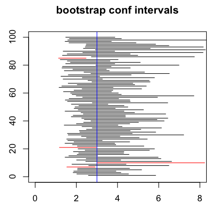
If I repeat this process from the start (including drawing a new x of 20 random exponential variables of mean 3) I can see how often the intervals actually contain the true mean. Here are 100 replicates of the whole interval creation process:

11 of the intervals, highlighted in red, do not contain the true mean 3, the blue vertical line. On average we would expect 5 if these are 95% confidence intervals. If I repeat this 1000 times, I get 88.4% of the intervals containing the true mean.
The bootstrap-t interval is a way of dealing with this problem. In An Introduction to the Bootstrap by Efron and Tibshirani, the authors write,
But it works well for calculating the mean, as in this case. This time we calculate a pivotal quantity as the bootstrapped statistic. For the vector x of random exponential variables of mean 3, we first calculate the mean and standard deviation of the original dataset:
Then for each bootstrap sample, calculate the difference between the mean and the bootstrap mean, divided by the standard deviation of the bootstrap.
Then to form a confidence interval, take quantiles of our bootstrapped statistic, multiply by the standard deviation of the original data and add this to the mean of the original data:
Now there are only 4 out of 100 intervals that do not contain the true mean:

If I do this 1000 times, I get 95.7% of the intervals containing the true mean. The mean interval size has increased though, from 2.4 for the simple intervals to 3.2 for the bootstrap-t intervals.
Here is an R script for this simulation.
Take 20 random exponential variables with mean 3. In R this looks like:
x = rexp(20,rate=1/3)Then generate B=1000 bootstrap samples of x, and calculate the mean for each bootstrap sample.
s = numeric(B)

for (j in 1:B) {

boot = sample(n,replace=TRUE)

s[j] = mean(x[boot])

}
Then, for an alpha = .05 / 95% confidence interval, look at the .025 and .975 quantiles of the bootstrap statistics in the vector s:
simple.ci = quantile(s,c(.025,.975))If I repeat this process from the start (including drawing a new x of 20 random exponential variables of mean 3) I can see how often the intervals actually contain the true mean. Here are 100 replicates of the whole interval creation process:

11 of the intervals, highlighted in red, do not contain the true mean 3, the blue vertical line. On average we would expect 5 if these are 95% confidence intervals. If I repeat this 1000 times, I get 88.4% of the intervals containing the true mean.
The bootstrap-t interval is a way of dealing with this problem. In An Introduction to the Bootstrap by Efron and Tibshirani, the authors write,
The quantity (theta-hat – theta)/se-hat is called an approximate pivot: this means that its distribution is approximately the same for each value of theta….Note the authors here are not comparing the bootstrap-t interval to the bootstrap percentile method. Also, they add a caveat: “The bootstrap-t method, at least in its simple form, cannot be trusted for more general problems, like setting a confidence interval for a correlation coefficient.”
Some elaborate theory shows that in large samples the coverage of the bootstrap-t interval tends to be closer to the desired level than the coverage of the standard interval or the interval based on the t table….
Notice also that the normal and t percentage points are symmetric about zero, and as a consequence the resulting intervals are symmetric about the point estimate theta-hat. In contrast, the bootstrap-t percentiles can be asymmetric about 0, leading to intervals which are longer on the left or right. This asymmetry represents an important part of the improvement in coverage it enjoys.
But it works well for calculating the mean, as in this case. This time we calculate a pivotal quantity as the bootstrapped statistic. For the vector x of random exponential variables of mean 3, we first calculate the mean and standard deviation of the original dataset:
x = rexp(n,rate=1/true.mean)

mean.x = mean(x)

sd.x = sd(x)
Then for each bootstrap sample, calculate the difference between the mean and the bootstrap mean, divided by the standard deviation of the bootstrap.
z = numeric(B)

for (j in 1:B) {

boot = sample(n,replace=TRUE)

z[j] = (mean.x - mean(x[boot]))/sd(x[boot])

}
Then to form a confidence interval, take quantiles of our bootstrapped statistic, multiply by the standard deviation of the original data and add this to the mean of the original data:
pivot.ci = mean.x + sd.x*quantile(z,c(.025,.975))Now there are only 4 out of 100 intervals that do not contain the true mean:

If I do this 1000 times, I get 95.7% of the intervals containing the true mean. The mean interval size has increased though, from 2.4 for the simple intervals to 3.2 for the bootstrap-t intervals.
Here is an R script for this simulation.
No comments:
Post a Comment
Thank you