R: Empirical Copulas and Hedge Basis Risk

Empirical Copulas and Hedge Basis Risk

October 10, 2011

The recently introduced proxy hedge model and corresponding empirical proxy quantiles share an implicit dependence on the joint covariation between underlying and proxy hedge. Of particular interest is understanding the dynamics of basis risk under extreme scenarios (both up and down), which are driven by time-varying stochastic joint covariation.
This post quantifies and visualizes such joint covariation and basis risk via copulas, including modeling and empirically fitting both marginal and joint distributions using fat-tailed student-t distributions. Copulas exploit multidimensional sample ranking, and thus are thematically similar to empirical quantiles. This analysis also seeks to exemplify practical use of R for copula analysis.

Brief review of the shortcomings of classic dependence statistics (such as correlation and covariance) motivates use of copulas and related techniques:

• Normality: assumption of joint normality in one guise or another, irrespective of suitability
• Summary statistics: point estimates which reduce complex covariation relationships into single numbers
• Marginal-joint conflation: considerations of both marginal and joint are conflated, rather than providing clean and independent separation
• Poor visualization: few visualization techniques exist, reducing potential for geometric and topological intuition

These shortcomings were resolved by the following beautiful decomposition, due to Sklar (1959):
   
where and are univariate distributions, is a two-dimensional distribution function with marginal distributions and , and is a copula. Note that any or all of , , and may be fitted empirically. Trivedi and Zimmer (2005) or Cherubini et al. (2004) are suggested for readers unfamiliar with copulas.
Conceptually, this technique provides several useful benefits for analyzing proxy hedging basis risk:

• Mechanics: Any joint distribution can be bi-directionally “glued together” by two marginals and a copula
• Uniqueness: Copula is unique, under conditions reasonable for current purposes
• Completeness: Joint covariation can be fully characterized by a copula, independent from the marginals
• Visualization: Copulas can graphically visualized, in both contours and density plots

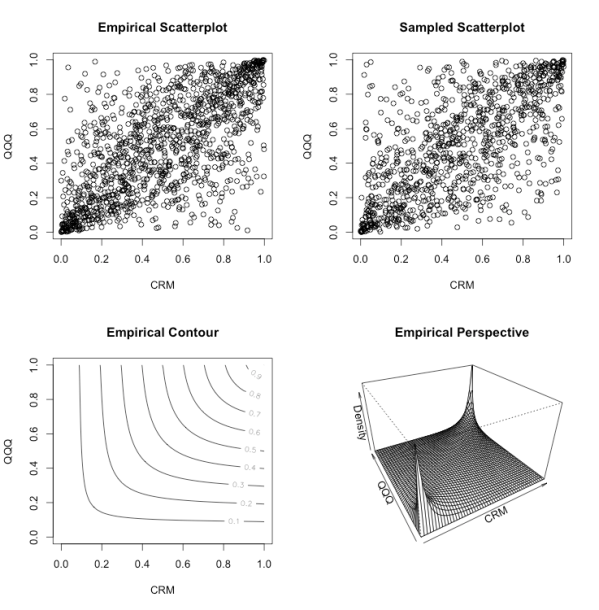
Without further ado, the following plots visualize the daily joint covariation of well-known tech stock and QQQ linear returns over the longitudinal period via an empirical proxy copula (1254 daily observations), as introduced in Empirical Quantiles and Proxy Selection. Note these plots illustrate joint covariation independent from the marginal densities of CRM / QQQ:

The top left plot illustrates scatter of ranked pseudo observations; top right illustrates scatter of 1000 random samples from the fitted copula; bottom left illustrates empirical copula contour; and bottom right illustrates the empirical copula perspective. Compare this diversity of visualization versus a single number (e.g. correlation statistic, which happens to equal 0.777).
Diving into the marginal and copula distribution is necessary to understand this relationship further. Consistent with standard convention, all distributions are assumed to be student-t with empirically fitted degrees of freedom. The parameters of the marginals are:
CRM location 0.0003 scale 0.0218 df 3.489
QQQ location 0.001 scale 0.0100 df 2.767
Indicating the marginal distributions diverge strongly from normality with fat trails, due to small degrees of freedom. This matches the 3 df estimate by Schoeffel in his recent (2011) article on futures (note difference in frequency and log returns).
Similarly, the copula is assumed to be distributed student-t with estimated df of 3.975 and of 0.6868. The bivariate association measures for the empirical proxy copula are:
tau 0.481
rho 0.669
tail index: 0.381 0.381
Indicating the copula also strongly diverges from normality with strongly fat tails.
In summary: these plots and fitted distributions confirm observed conclusions from the previous post: although CRM and QQQ covary, there is high basis risk—including numerous observations with nearly inverse correlation. In other words, a QQQ proxy is likely to result in fairly costly hedging errors.

---

R code to generate the above empirical proxy copula analysis (and more, possibly to be covered in a subsequent post):

001	require("copula")

002	require("fSeries")

003

004	exploreProxyDist <- function(p, doExcess=TRUE, partitions=1)

005

{

006	# Analyze distribution and copula of proxy daily returns.

007

#

008

# Args:

009	#   p: matrix of instrument price data, including valid colnames

010	#   doExcess: flag indicating whether to perform analysis on excess returns,

011	#             in addition to raw returns

012	#   partitions: if not 1, partition the returns and perform subanalysis

013

#

014	# Returns: None

015

016	oldpar <- par(mfrow=c(2,2))

017	n <- nrow(p)

018

019	# first differences (not logged)

020	pROC <- ROC(p, type="discrete", na.pad=FALSE)

021	exploreProxyDistROC(pROC)

022

023	if (partitions > 1)

024

{

025	frac <- floor(n / partitions)

026	sapply(c(0:(partitions-1)), function(p) { cat("\n",

027	(p+1),"-th partition:",((p*frac)+1),

028	((p+1)*frac),"\n");

029	partition <- pROC[((p*frac)+1):((p+1)*frac),]

030	exploreProxyDistROC(partition) } )

031

}

032

033	if (doExcess)

034

{

035	cat("\nExcess Copula\n")

036

037	# calculate excess returns, subtracting off market

038	excess <- pROC[,1] - pROC[,2]

039	excessROC <- cbind(excess, pROC[,2])

040

041	par(oldpar)

042	plot(cumprod(1+excess), main="Excess Cumulative Returns", ylab="Return")

043	oldpar <- par(mfrow=c(2,2))

044

045	exploreProxyDistROC(excessROC)

046

047	if (partitions > 1)

048

{

049	frac <- floor(n / partitions)

050	sapply(c(0:(partitions-1)), function(p) { cat("\n",

051	(p+1),"-th Excess Partition:",((p*frac)+1),

052	((p+1)*frac),"\n");

053	partition  <- excessROC[((p*frac)+1):((p+1)*frac),]

054	exploreProxyDistROC(partition) } )

055

}

056

}

057

058	par(oldpar)

059

}

060

061	exploreProxyDistROC <- function(pROC)

062

{

063	# Analyze distribution and copula of proxy daily returns.

064

#

065

# Args:

066	#   p: matrix of instrument price data, including valid colnames

067

#

068	# Returns: list of copula fit and empirical copula

069

070	n <- nrow(pROC)

071	cnames <- colnames(pROC)

072

073	# t-distribution fits

074	p1Fit <- fitdistr(pROC[,1], "t")$estimate

075	p2Fit <- fitdistr(pROC[,2], "t")$estimate

076

077	cat(cnames[1], "location", p1Fit[1], "scale", p1Fit[2], "df", p1Fit[3], "\n")

078	cat(cnames[2], "location", p2Fit[1], "scale", p2Fit[2], "df", p2Fit[3], "\n")

079

080	# empirical copula

081	tau <- cor(pROC, method="kendall")[2]

082	t.cop <- tCopula(tau, dim=2, dispstr="un", df=3)

083	psuedo <- apply(pROC, 2, rank) / (n + 1)

084	plot(psuedo, main="Empirical Scatterplot", xlab=cnames[1], ylab=cnames[2])

085

086	fit.mpl <- fitCopula(t.cop, psuedo, method="mpl", estimate.variance=FALSE)

087	print(fit.mpl)

088

089

090	# build empirical copula and plot

091	empiricalCopula <- tCopula(fit.mpl@estimate[1], dim=2, dispstr="un", df=fit.mpl@estimate[2])

092	plot(rcopula(empiricalCopula, 1000), main="Sampled Scatterplot", xlab=cnames[1], ylab=cnames[2])

093	contour(empiricalCopula, pcopula, main="Empirical Contour", xlab=cnames[1], ylab=cnames[2])

094	persp(empiricalCopula, dcopula, main="Empirical Perspective",

095	xlab=cnames[1], ylab=cnames[2], zlab="Density")

096

097	cat("Empirical tau:", kendallsTau(empiricalCopula), "\n")

098	cat("Empirical rho:", spearmansRho(empiricalCopula), "\n")

099	cat("Empirical tail index:", tailIndex(empiricalCopula), "\n")

100

101	return (list(fit=fit.mpl, copula=empiricalCopula))

102

}